日记-20221121
Xwyturbo / 2022-11-21
不开心的是小徐的工作被重置了,但师门的人都是非常nice的。

library(readxl)
library(tidyverse)
## ── Attaching packages ─────────────────────────────────────── tidyverse 1.3.2 ──
## ✔ ggplot2 3.3.6      ✔ purrr   0.3.5
## ✔ tibble  3.1.8      ✔ dplyr   1.0.10
## ✔ tidyr   1.2.1      ✔ stringr 1.4.1
## ✔ readr   2.1.3      ✔ forcats 0.5.2
## ── Conflicts ────────────────────────────────────────── tidyverse_conflicts() ──
## ✖ dplyr::filter() masks stats::filter()
## ✖ dplyr::lag()    masks stats::lag()
library(writexl)
library(ggplot2)
library(ggpubr)
library(patchwork)
library(factoextra)
## Warning: package 'factoextra' was built under R version 4.2.2
## Welcome! Want to learn more? See two factoextra-related books at https://goo.gl/ve3WBa
suide <- read_xls("D:/suide_1121/excel/land_clip_check_Statistics1_TableToExcel_1.xls")
str(suide)
## tibble [6,104 × 3] (S3: tbl_df/tbl/data.frame)
##  $ XZQDM   : chr [1:6104] "610826100003" "610826100003" "610826100003" "610826100003" ...
##  $ DLMC    : chr [1:6104] "城镇村道路用地" "城镇住宅用地" "公路用地" "灌木林地" ...
##  $ SUM_TBMJ: num [1:6104] 123.8 4061.3 83.2 24.9 1843.8 ...
#  长表转宽表
suide01 <- suide %>%
  pivot_wider(names_from = DLMC, values_from = SUM_TBMJ, values_fill = 0)
str(suide01)
## tibble [341 × 39] (S3: tbl_df/tbl/data.frame)
##  $ XZQDM               : chr [1:341] "610826100003" "610826100200" "610826100201" "610826100202" ...
##  $ 城镇村道路用地      : num [1:341] 124 1571 673 0 459 ...
##  $ 城镇住宅用地        : num [1:341] 4061.33 11198.35 11740.22 0 6.21 ...
##  $ 公路用地            : num [1:341] 83.2 182.6 396.6 0 247.4 ...
##  $ 灌木林地            : num [1:341] 24.9 83.8 295.4 3175.7 1401.5 ...
##  $ 果园                : num [1:341] 1844 588 3530 21528 1743 ...
##  $ 旱地                : num [1:341] 126 117 1238 2420 839 ...
##  $ 河流水面            : num [1:341] 347.2 1001.7 1873.8 76.8 589 ...
##  $ 机关团体新闻出版用地: num [1:341] 3.53 525.99 142.96 0 149.42 ...
##  $ 科教文卫用地        : num [1:341] 409 502 1687 0 298 ...
##  $ 裸土地              : num [1:341] 9.64 0 10.72 27.7 68.2 ...
##  $ 农村道路            : num [1:341] 23.5 45.4 408.7 541.2 168.8 ...
##  $ 其他草地            : num [1:341] 755 418 4900 12248 1721 ...
##  $ 其他林地            : num [1:341] 124 365 6512 7206 5305 ...
##  $ 设施农用地          : num [1:341] 6.02 0 66.03 7.6 25.28 ...
##  $ 特殊用地            : num [1:341] 294 110 652 0 223 ...
##  $ 天然牧草地          : num [1:341] 127.2 44.9 3599.3 7680.4 5272.8 ...
##  $ 公用设施用地        : num [1:341] 0 157.02 25.92 0 4.83 ...
##  $ 公园与绿地          : num [1:341] 0 155.36 5.94 0 0 ...
##  $ 交通服务场站用地    : num [1:341] 0 236.79 7.97 0 30.75 ...
##  $ 空闲地              : num [1:341] 0 144 0 0 62 ...
##  $ 内陆滩涂            : num [1:341] 0 2103 377 0 734 ...
##  $ 农村宅基地          : num [1:341] 0 21.4 262 987.5 4490.9 ...
##  $ 乔木林地            : num [1:341] 0 61 81.8 628.1 0 ...
##  $ 商业服务业设施用地  : num [1:341] 0 733 306 0 415 ...
##  $ 水工建筑用地        : num [1:341] 0 335.5 64.3 0 172.6 ...
##  $ 水浇地              : num [1:341] 0 10.1 0 0 0 ...
##  $ 工业用地            : num [1:341] 0 0 110 0 217 ...
##  $ 沟渠                : num [1:341] 0 0 33.1 0 0 ...
##  $ 广场用地            : num [1:341] 0 0 48.7 0 4.29 ...
##  $ 其他园地            : num [1:341] 0 0 1419 328 0 ...
##  $ 坑塘水面            : num [1:341] 0 0 0 18.1 14.6 ...
##  $ 铁路用地            : num [1:341] 0 0 0 0 5.57 ...
##  $ 物流仓储用地        : num [1:341] 0 0 0 0 64 ...
##  $ 采矿用地            : num [1:341] 0 0 0 0 0 ...
##  $ 裸岩石砾地          : num [1:341] 0 0 0 0 0 ...
##  $ 管道运输用地        : num [1:341] 0 0 0 0 0 0 0 0 0 0 ...
##  $ 养殖坑塘            : num [1:341] 0 0 0 0 0 0 0 0 0 0 ...
##  $ 人工牧草地          : num [1:341] 0 0 0 0 0 0 0 0 0 0 ...
sd_data <- tibble(XZQDM = suide01$XZQDM,
                  科教文卫用地 = suide01$科教文卫用地,
                  交通运输用地 = suide01$公路用地+suide01$交通服务场站用地+
                    suide01$铁路用地+suide01$管道运输用地,
                  林地 = suide01$其他林地+suide01$灌木林地+suide01$乔木林地,
                  园地 = suide01$果园+suide01$其他园地,
                  水域及水利设施 = suide01$河流水面+
                    suide01$内陆滩涂+suide01$水工建筑用地+suide01$沟渠+
                    suide01$坑塘水面+suide01$养殖坑塘,
                  旱地 = suide01$旱地,
                  草地 = suide01$其他草地+suide01$天然牧草地+suide01$人工牧草地,
                  水浇地 = suide01$水浇地,
                  设施农用地 = suide01$设施农用地,
                  矿业用地 = suide01$采矿用地,
                  公共服务用地 = suide01$机关团体新闻出版用地+suide01$公用设施用地+
                    suide01$公园与绿地+suide01$广场用地,
                  商服用地 = suide01$商业服务业设施用地,
                  工业用地 = suide01$工业用地,
                  物流仓储用地 = suide01$物流仓储用地)

sd_14_mianji <- sd_data[,2:15]
#  计算每个村庄每种地类的占村庄全部用地的比重。
sd1 <- sd_14_mianji/rowSums(sd_14_mianji)
#  计算县域范围内每种地类占全部用地的比重
sd2 <- colSums(sd_14_mianji)/sum(sd_14_mianji)

sd_14_quweishang <- tibble(
  x1 = sd1$科教文卫用地/sd2[1],
  x2 = sd1$交通运输用地/sd2[2],
  x3 = sd1$林地/sd2[3],
  x4 = sd1$园地/sd2[4],
  x5 = sd1$水域及水利设施/sd2[5],
  x6 = sd1$旱地/sd2[6],
  x7 = sd1$草地/sd2[7],
  x8 = sd1$水浇地/sd2[8],
  x9 = sd1$设施农用地/sd2[9],
  x10 = sd1$矿业用地/sd2[10],
  x11 = sd1$公共服务用地/sd2[11],
  x12 = sd1$商服用地 /sd2[12],
  x13 = sd1$工业用地/sd2[13],
  x14 = sd1$物流仓储用地/sd2[14]
)

sd <- cbind(sd_data,sd_14_quweishang)
str(sd)
## 'data.frame':	341 obs. of  29 variables:
##  $ XZQDM         : chr  "610826100003" "610826100200" "610826100201" "610826100202" ...
##  $ 科教文卫用地  : num  409 502 1687 0 298 ...
##  $ 交通运输用地  : num  83.2 419.4 404.5 0 283.8 ...
##  $ 林地          : num  149 510 6889 11010 6707 ...
##  $ 园地          : num  1844 588 4950 21856 1743 ...
##  $ 水域及水利设施: num  347.2 3439.9 2348.4 94.9 1510.4 ...
##  $ 旱地          : num  126 117 1238 2420 839 ...
##  $ 草地          : num  882 463 8499 19928 6994 ...
##  $ 水浇地        : num  0 10.1 0 0 0 ...
##  $ 设施农用地    : num  6.02 0 66.03 7.6 25.28 ...
##  $ 矿业用地      : num  0 0 0 0 0 ...
##  $ 公共服务用地  : num  3.53 838.37 223.53 0 158.54 ...
##  $ 商服用地      : num  0 733 306 0 415 ...
##  $ 工业用地      : num  0 0 110 0 217 ...
##  $ 物流仓储用地  : num  0 0 0 0 64 ...
##  $ x1            : num  182.5 113.1 108.4 0 26.5 ...
##  $ x2            : num  3.53 9 2.47 0 2.41 ...
##  $ x3            : num  0.259 0.448 1.727 1.333 2.333 ...
##  $ x4            : num  2.353 0.379 0.91 1.941 0.445 ...
##  $ x5            : num  6.186 30.956 6.027 0.118 5.38 ...
##  $ x6            : num  0.1576 0.0744 0.2238 0.2114 0.2105 ...
##  $ x7            : num  0.567 0.15 0.787 0.892 0.899 ...
##  $ x8            : num  0 0.118 0 0 0 ...
##  $ x9            : num  2.097 0 3.315 0.184 1.761 ...
##  $ x10           : num  0 0 0 0 0 ...
##  $ x11           : num  1.46 174.87 13.3 0 13.09 ...
##  $ x12           : num  0 109.7 13.1 0 24.6 ...
##  $ x13           : num  0 0 5.42 0 14.8 ...
##  $ x14           : num  0 0 0 0 42.9 ...
#   write_xlsx(sd,"14种地类面积与区位商的分村计算结果.xlsx")
#  宽表转长表

sd_mjlong = sd[,1:15] %>%
  pivot_longer(-XZQDM, names_to = "地类", values_to = "面积/公亩")
str(sd_mjlong)
## tibble [4,774 × 3] (S3: tbl_df/tbl/data.frame)
##  $ XZQDM    : chr [1:4774] "610826100003" "610826100003" "610826100003" "610826100003" ...
##  $ 地类     : chr [1:4774] "科教文卫用地" "交通运输用地" "林地" "园地" ...
##  $ 面积/公亩: num [1:4774] 409 83.2 149 1843.8 347.2 ...
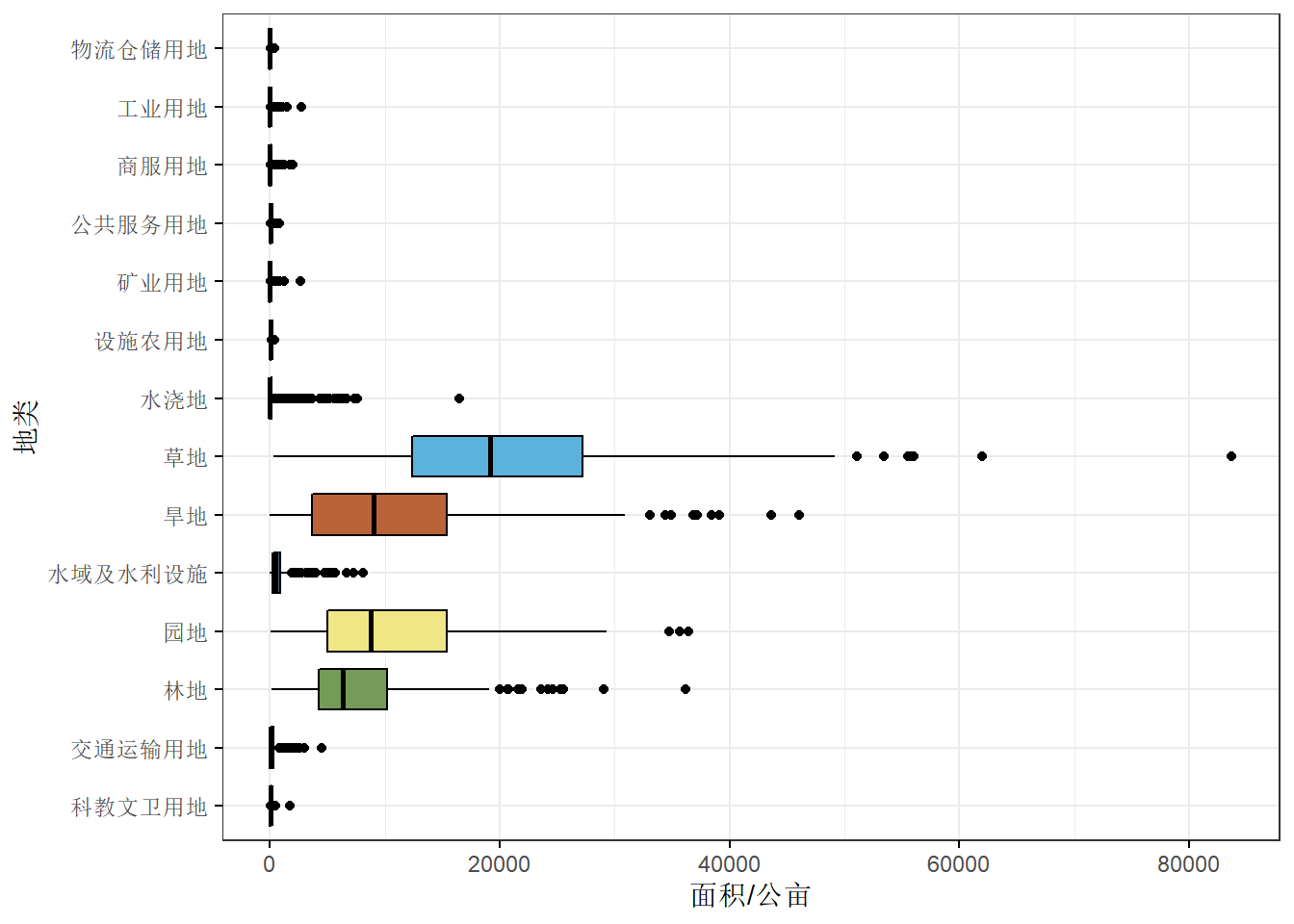
# 14种地类面积箱线图
p1 <- ggboxplot(sd_mjlong, x="地类", y="面积/公亩",fill ="地类",
                palette = "igv",
                sorting = "descending",
                rotate = TRUE,
                ggtheme = theme_bw())+
  theme(legend.position = "none")
p1
# ggexport(p1,filename = "pics/14种地类面积箱线图.png",
#          width = 4000,height = 2000,
#          res = 600)

#  宽表转长表

sd_qws<-sd[,c(1,16:29)]
names(sd_qws) <- c("XZQDM",
  "科教文卫用地","交通运输用地","林地",
  "园地","水域及水利设施","旱地","草地",
  "水浇地","设施农用地","矿业用地",
  "公共服务用地","商服用地",
  "工业用地","物流仓储用地")
sd_qwslonger = sd_qws %>%
  pivot_longer(-XZQDM, names_to = "地类", values_to = "区位商")
str(sd_qwslonger)
## tibble [4,774 × 3] (S3: tbl_df/tbl/data.frame)
##  $ XZQDM : chr [1:4774] "610826100003" "610826100003" "610826100003" "610826100003" ...
##  $ 地类  : chr [1:4774] "科教文卫用地" "交通运输用地" "林地" "园地" ...
##  $ 区位商: num [1:4774] 182.459 3.532 0.259 2.353 6.186 ...
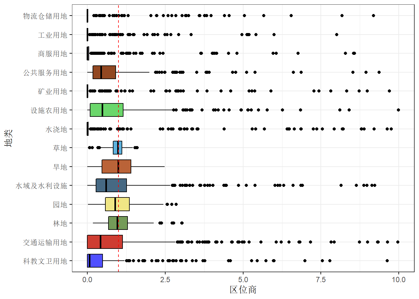
p2 <- ggboxplot(sd_qwslonger, x="地类", y="区位商",fill ="地类",
                palette = "igv",
                sorting = "descending",
                rotate = TRUE,
                ggtheme = theme_bw())+
  theme(legend.position = "none")+
  geom_hline(yintercept = 1,linetype = 2,
             color = "red")+
  ylim(0,10)
p2
## Warning: Removed 105 rows containing non-finite values (stat_boxplot).
# ggexport(p2,filename = "pics/14种地类区位商箱线图.png",
# width = 4000,height = 2000,
# res = 600)
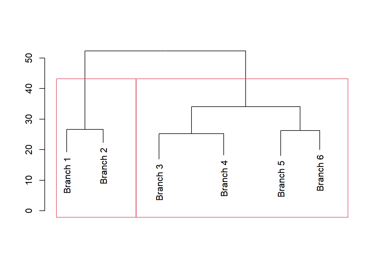
# 层次聚类
d <- dist(sd[,16:29],"canberra")
hc <- hclust(d,"ward.D2")
tree = as.dendrogram(hc)
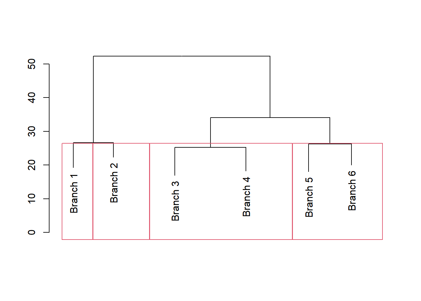
c2 <- cutree(hc,2)
table(c2)
## c2
##   1   2
##  93 248
plot(cut(tree, h=25)$upper, horiz=FALSE)
rect.hclust(hc,2)
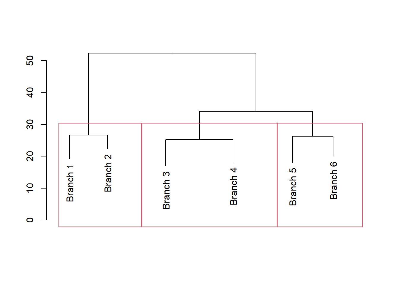
c3 <- cutree(hc,3)
table(c3)
## c3
##   1   2   3
##  93  96 152
plot(cut(tree, h=25)$upper, horiz=FALSE)
rect.hclust(hc,3)
c4 <- cutree(hc,4)
table(c4)
## c4
##   1   2   3   4
##  33  60  96 152
plot(cut(tree, h=25)$upper, horiz=FALSE)
rect.hclust(hc,4)
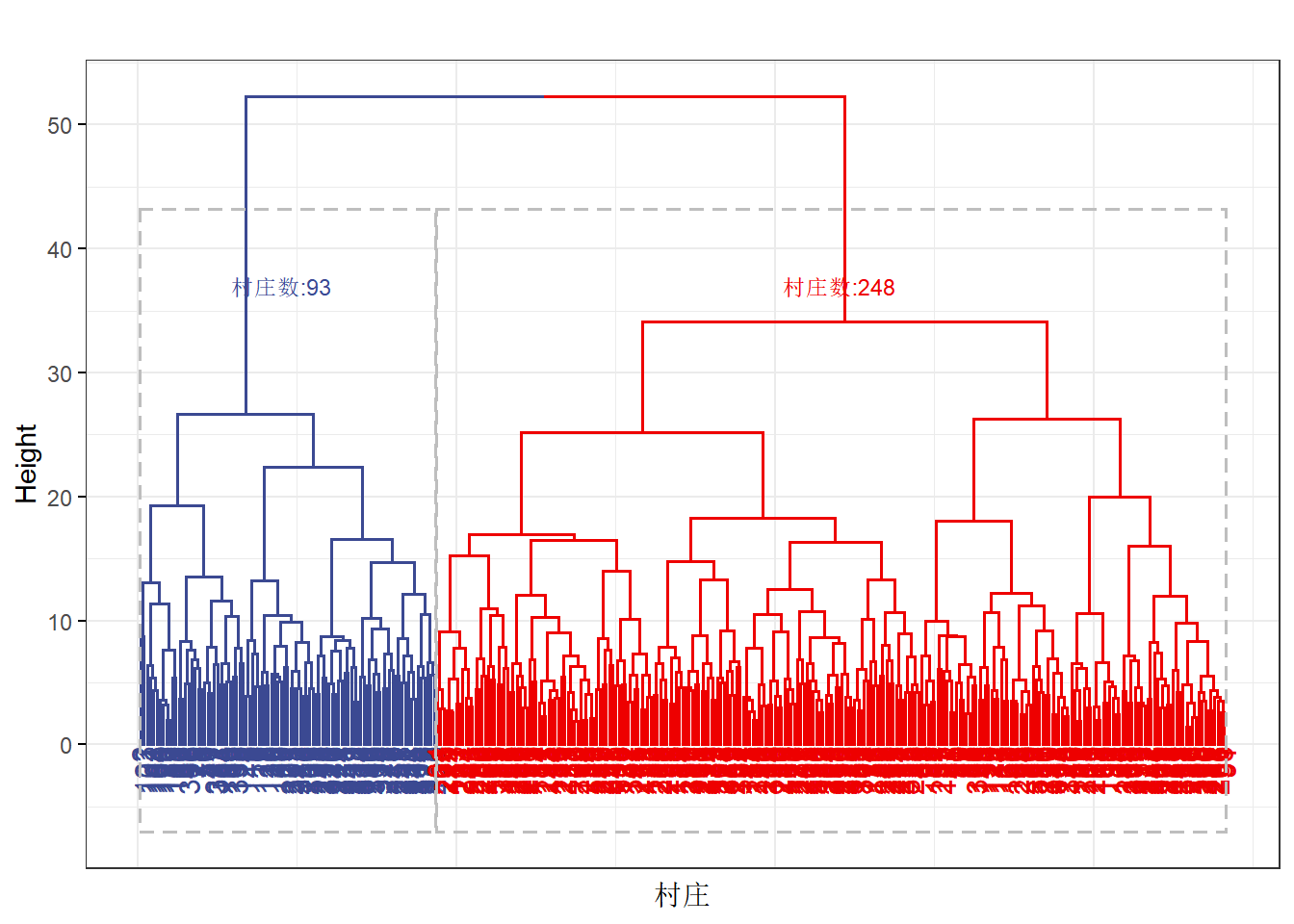
p42 <- fviz_dend(hc,k = 2,
                 xlab = "村庄",
                 ylab = "Height",
                 main = "",
                 rect = TRUE,
                 k_colors = c("#3B4992FF","#EE0000FF"),
                 ggtheme = theme_bw())+
  annotate("text", x = 45, y = 37,label = "村庄数:93",colour= "#3B4992FF",size=3)+
  annotate("text", x = 220, y = 37,label = "村庄数:248",colour= "#EE0000FF",size=3)
## Warning: `guides(<scale> = FALSE)` is deprecated. Please use `guides(<scale> =
## "none")` instead.
p42
# ggexport(p42,filename = "pics/聚类谱系图2.png",
# width = 3400,height = 3000,
# res = 600)
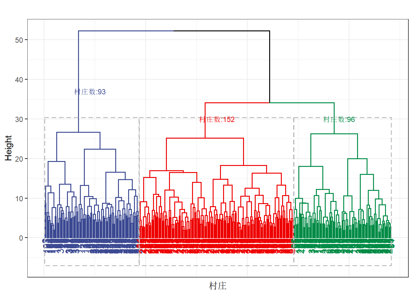
p43 <- fviz_dend(hc,k = 3,
xlab = "村庄",
ylab = "Height",
main = "",
rect = TRUE,
k_colors = c("#3B4992FF","#EE0000FF","#008B45FF"),
ggtheme = theme_bw())+
annotate("text", x = 45, y = 37,label = "村庄数:93",colour= "#3B4992FF",
size = 3)+
annotate("text", x = 170, y = 30,label = "村庄数:152",colour= "#EE0000FF",
size = 3)+
annotate("text", x = 290, y = 30,label = "村庄数:96",colour= "#008B45FF",
size = 3)
## Warning: `guides(<scale> = FALSE)` is deprecated. Please use `guides(<scale> =
## "none")` instead.
p43
# ggexport(p43,filename = "pics/聚类谱系图3.png",
# width = 3400,height = 3000,
# res = 600)
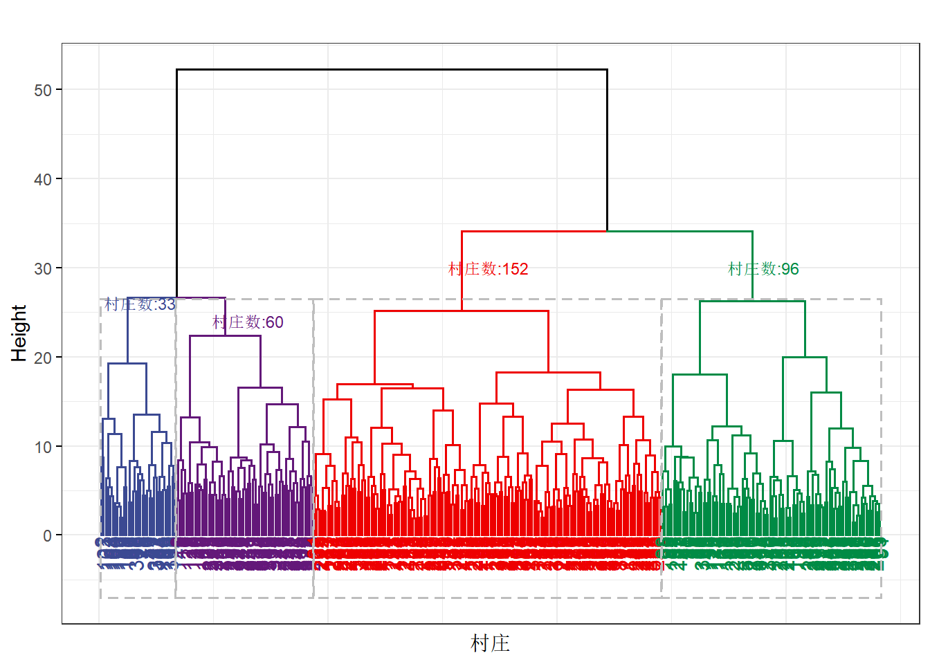
p44 <- fviz_dend(hc,k = 4,
xlab = "村庄",
ylab = "Height",
main = "",
rect = TRUE,
k_colors = c("#3B4992FF","#631879FF","#EE0000FF","#008B45FF"),
ggtheme = theme_bw())+
annotate("text", x = 65, y = 24,label = "村庄数:60",colour= "#631879FF",
size = 3)+
annotate("text", x = 170, y = 30,label = "村庄数:152",colour= "#EE0000FF",
size = 3)+
annotate("text", x = 290, y = 30,label = "村庄数:96",colour= "#008B45FF",
size = 3)+
annotate("text", x = 18, y = 26,label = "村庄数:33",colour = "#3B4992FF",
size = 3)
## Warning: `guides(<scale> = FALSE)` is deprecated. Please use `guides(<scale> =
## "none")` instead.
p44
# ggexport(p44,filename = "pics/聚类谱系图3.png",
#          width = 3400,height = 3000,
#          res = 600)

#  "#3B4992FF","#631879FF","#EE0000FF","#008B45FF" 蓝色、紫色、红色、绿色

#  "#3B4992FF","#EE0000FF","#008B45FF" 蓝色、红色、绿色

#  "#3B4992FF","#EE0000FF";  蓝色、红色